Intro

Basically every machine learning AI problem is now solved using deep learning. Deep learning is the approach of using neural networks to learn from data, in this approach we don’t need to decide on what the model (neural network) should do, we just need to give it the data and the model will learn to do the task.

At its core, deep learning relies on lots of data and the concept of high dimensional features (more below). This is a first blog post covering the fundamental building blocks of deep learning.

Learning from Data

All of AL and ML uses lots and lots of data. Without it you can’t really get anywhere. So what actually happens when we learn from data? Well, what we want is to learn a model (Neural Network) that can map inputs to outputs. A great example is the MNIST dataset, which is a dataset of handwritten digits. We want to learn a model that can map an image of a handwritten digit to the correct digit. To do this, we create a model and then repeatedly show the data to the model, given that we know the correct answers (the digit). We can then adjust the model based on the data it got wrong.

This process is known as training the model. Where we evaluate how corret the model is using a loss function, and then adjust the model by changing the parameters (millions of numbers that describe the model) based on the loss function. We know how to change the parameters by taking the gradient of the loss function, this tells us how to change the parameters to get a better model.

This will all make sense soon, I promise.

Fundamentals of Deep Learning

Vectors

AI is based on high dimensions, and what I mean by this is having many ways that you can change a number to get many combinations. If we look at a single number we can only change it in one way, but if we look at a vector we can change it in many ways.

Looking at the first vector we can change $x_1$ and $x_2$ to get many combinations. But if we look at the second vector we can change $x_1$, $x_2$ and $x_3$ to get even more combinations of $\mathbf{x}$. This is exactly why we use vectors in deep learning, we can create many vectors that represent the complexities and nuances of the data, such as images of numbers.

Features

If you are interested in computer vision you will have heard the term features a lot. Confusingly features can mean two things: 1. the actualy parts of the image that make something a class (e.g. the face of the cat) and 2. the vectors that the model learns to extract from the data. It’s always good to clarify what someone means by features, do they mean in the data or in the model?

Neural Networks

A neural network consists of many layers which each transform the data in some way. The fundamental building block is the fully connected layer, mathematically represented as:

\(\mathbf{y} = \sigma(\mathbf{W} \mathbf{x} + \mathbf{b})\) where:

$\mathbf{x}$ is the input vector,
$\mathbf{W}$ is the weight matrix,
$\mathbf{b}$ is the bias vector,
$\sigma(\cdot)$ is a nonlinear activation function.

What this does is transform our input vector $\mathbf{x}$. Specifically, it takes $\mathbf{x}$ and then multiplies it by the weight matrix $\mathbf{W}$, adds the bias vector $\mathbf{b}$, and then finally applies the activation function $\sigma(\cdot)$.

This process is repeated for each layer in the network, and the output of one layer is used as the input to the next layer.

Activation Functions

We introduced the activation function $\sigma(\cdot)$ in the previous section. This is a function that takes a vector and applies a nonlinear transformation to it. This is important because it allows us to learn more complex models.

There are many different activation functions, but some of the most common ones are:

Sigmoid: \(\sigma(x) = \frac{1}{1 + e^{-x}}\)

ReLU (Rectified Linear Unit): \(f(x) = \max(0, x)\)

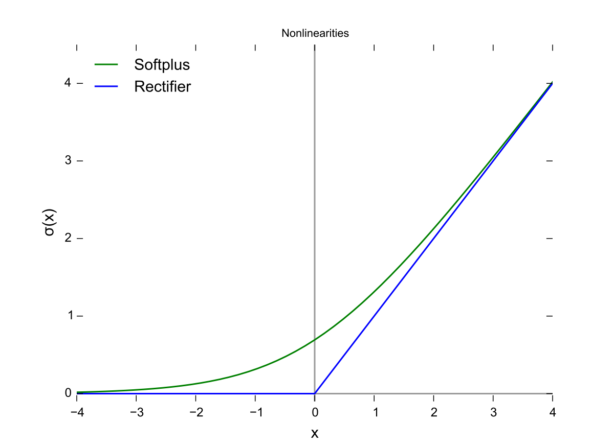
Softmax (for multi-class classification): \(\sigma(\mathbf{x})_i = \frac{e^{x_i}}{\sum_{j} e^{x_j}}\)

If we have two outputs, then the softmax becomes the sigmoid.

Convolutional Neural Networks (CNNs)

The Convolution Operation

The issue with fully connected layers is that they are sensitive to the location of the feature in the data. If our trainig data always shows birds in the sky, then the model will learn to only classify birds in the top half of the image.

This is where convolutional layers come in. Like fully connected layers convolutional layers are a type of layer that is used to extract features from the data. But they are invariant to the location of the feature in the data. They do this by using a filter/kernal which is a small matrix of weights that we slide over the image to get the feature.

\(Y(i, j) = \sum_m \sum_n K(m, n) X(i - m, j - n)\) where:

$X(i,j)$ is the input pixel,
$K(m,n)$ is the filter,
$Y(i,j)$ is the output at position $(i,j)$.

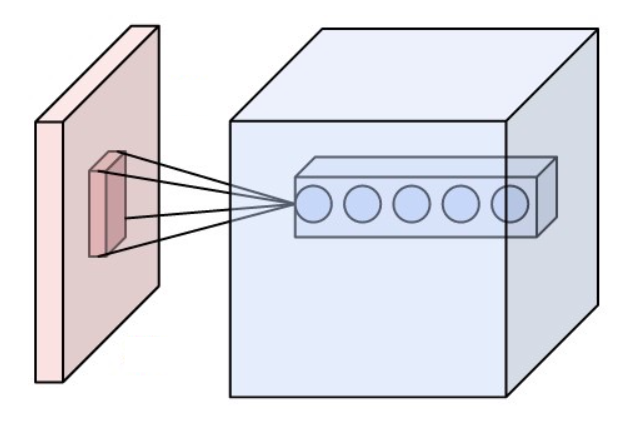
Figure: A visual representation of the convolution operation. The filter (kernel) is applied to the input image, resulting in an output feature map. Image from Wikimedia Commons.

Pooling Layers:
Max Pooling:

ResNet: Deep Residual Networks

One issue that happens when you train a neural network is that the gradient (our signal on how to change the parameters) can become 0, meaning we can’t learn anything. To get around this, ResNet introduced residual connections. These are basically a shortcut from the input to the output. It’s quite amazing about how successful they were, basically every model pre-2022 used some sort of skip connection.

\(\mathbf{y} = F(\mathbf{x}) + \mathbf{x}\) A basic ResNet block is:

i.e. we basically add the input to the output, this allows the gradient to flow directly through the network.

Figure: A ResNet block showing the skip connection (shortcut) that allows gradients to flow directly through the network. The main path consists of convolutional layers with batch normalization and ReLU activation. Image from He et al. 2015

U-Net

The other popular architecture in the field of computer vision is U-Net. It’s a type of convolutional neural network that is used when we want the output to have the same size as the input. It’s a type of encoder-decoder architecture. It basically consists of a contracting path and an expanding path.

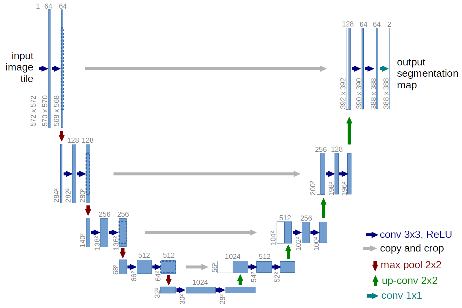
Figure: U-Net architecture showing the contracting path (left) and expansive path (right). Image from Ronneberger et al. 2015

Training a Neural Network

Training a deep neural network involves optimizing (finding the best) parameters to minimize a loss function (how wrong the model is). The most common approach is gradient descent.

Loss Function

A typical loss function for classification tasks is the cross-entropy loss:

\(L = - \sum_{i} y_i \log \hat{y}_i\) where:

$y_i$ is the true label,
$\hat{y}_i$ is the predicted probability.

This loss function will return a single number that tells us how wrong the model is. If it is high then the model is doing poorly, if it is low then the model is doing well. We want to find the parameters that minimize this loss function.

Gradient Descent and Backpropagation

Gradient Descent is a method that finds the minimum of a function. It works by taking the gradient of the loss function and then updating the parameters in the opposite direction of the gradient. This is because the gradient points in the direction of the steepest ascent, so by going in the opposite direction we move towards the minimum. A great analogy is if you are on a hill and you want to find the coordinates of the bottom, you look around and take a step in the direction that is steepest downhill. It’s the same with optimizing a neural network, we want to find the parameters that minimize the loss function, rather than the coordinates of the bottom of the hill.

The weight update rule in gradient descent:

Like walking down the hill, we take several steps in the direction that is steepest downhill.

Algorithm: Gradient Descent

Input: Training data ${\mathbf{X}, \mathbf{y}}$, learning rate $\eta$, max epochs $T$, convergence threshold $\epsilon$

Output: Optimized parameters $\mathbf{w}$

Algorithm:

1. Initialize $\mathbf{w}^{(0)}$ randomly
2. Set $t = 0$
3. While $t < T$:
   1. Forward pass:
      • Compute predictions: $\hat{\mathbf{y}} = f(\mathbf{X}; \mathbf{w}^{(t)})$
      • Compute loss: $L^{(t)} = -\sum_i y_i \log \hat{y}_i$
   2. Backward pass:
      • Compute gradients: $\mathbf{g}^{(t)} = \nabla_{\mathbf{w}} L(\mathbf{w}^{(t)})$
   3. Update parameters:
      • $\mathbf{w}^{(t+1)} = \mathbf{w}^{(t)} - \eta \mathbf{g}^{(t)}$
   4. $t = t + 1$
4. Return $\mathbf{w}^{(t)}$

Note: The convergence check starts after the first iteration ($t > 0$) since $L^{(t-1)}$ doesn’t exist for $t=0$.

Here epochs is the number of times we pass through the data. and $\eta$ is the learning rate that controls how big of a step we take in the direction of the gradient.

Summary

That’s it! You now know the fundamental building blocks of deep learning. In the next blog post we will dig more into the math and details of why this works.