Loss Landscapes

In the last post we spoke about walking down the hill to find the location of the lowest point. This is a great analogy for training a neural network, we want to find the parameters that minimize the loss function. You can think of the loss function as the height of the hill, and the parameters as the coordinates of the hill. This landscape is called the loss landscape, and we talk alot about it in the deep learning community. Specifically in relation to valleys, local minima, saddle points, and flat regions. Whenever you hear these terms, just think about hills and valleys.

Here’s a visualization of a real neural network’s loss landscape:

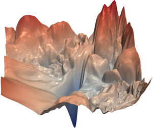
This visualization comes from the paper “Visualizing the Loss Landscape of Neural Nets” (Li et al., 2018). The plot shows the loss surface of a ResNet-56 neural network trained on CIFAR-10. The valleys, peaks, and contours represent different loss values as the network’s parameters change. The relatively smooth areas indicate regions where training can proceed effectively, i.e. you can walk down the hill. But the the sharp peaks and valleys show areas where training might become unstable, i.e. you would fall off a cliff. This kind of visualization has been instrumental in understanding why deep neural networks can be challenging to train and why certain architectures train more successfully than others.

Training Dynamics

When training neural networks, we encounter various phenomena that affect how well and how quickly the network learns. Let’s explore some key concepts in training dynamics:

Local Minima and Global Minima

A local minimum is a point where the loss is lower than all nearby points, but may not be the lowest possible value (global minimum). Early concerns about local minima hampering neural network training have largely been addressed by research showing that in high-dimensional spaces, most local minima are actually quite good solutions. The real challenge often lies elsewhere.

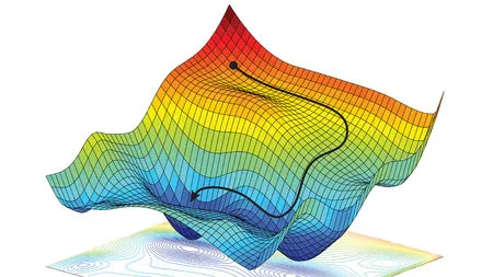
The figure above shows a 2D loss landscape with both local and global minima. The local minimum represents a point where the loss is lower than its immediate surroundings but not the lowest possible value. The global minimum represents the lowest possible loss value in the entire landscape. In practice, neural networks operate in much higher dimensional spaces, but this 2D visualization helps build intuition about these important concepts.

Saddle Points

Saddle points are locations where the gradient is zero, but they’re neither minima nor maxima - imagine a mountain pass between two peaks. These are actually more common than local minima in high-dimensional spaces and can significantly slow down training as optimizers can get “stuck” here temporarily. This is one reason why momentum-based optimizers are helpful - they can help push through these flat regions.

A saddle point in 3D, showing the characteristic “mountain pass” shape. From one direction it looks like a maximum (going up), while from another direction it looks like a minimum (going down). This geometry makes it challenging for optimizers, as the gradient is zero at this point despite it not being a minimum.

Gradient Issues

Several gradient-related challenges can affect training:

1. Vanishing Gradients: When gradients become extremely small, parameters barely update, making learning very slow or impossible. This often happens in deep networks, especially with certain activation functions like sigmoid. Here we can be at a local minimum, but it’s a very bad one. This if often why we use ReLU activation functions.

2. Exploding Gradients: The opposite problem - when gradients become very large, causing unstable training with dramatic parameter updates, like falling off a cliff. This can make the network “bounce” around the loss landscape, never converging to a good solution. This is often why we use gradient clipping, and can be thought of as slowly climbing down the cliff.

Learning Rate Dynamics

The learning rate plays a crucial role in training dynamics:

• Too large: The network might overshoot and lead to a bad outcome, like jumping too far down the hill/cliff
• Too small: Training becomes very slow and might get stuck in poor local optima, we might not be moving fast enough
• Just right: The network converges efficiently to a good solution. Typically we use learning rates that are between 0.001 and 0.00001.

This is why learning rate scheduling (gradually adjusting the learning rate during training) has become a common practice in deep learning.

Jacobian and Hessian in Deep Learning

The Jacobian and Hessian matrices are mathematical tools used to analyze the behavior of the loss landscape. In short they represent the steeness of the loss landscape and how quickly it changes.

Jacobian Matrix

The Jacobian matrix is used to describe the rate of change of the output of a neural network with respect to its inputs, i.e. how steep the loss landscape is at a point. It is particularly useful in understanding how small changes in input can affect the output, which is crucial for tasks like sensitivity analysis and adversarial attacks (more later).

The Jacobian, will give a vector (a direction) of the steepest direction up the loss landscape.

The figure above illustrates the steepness of gradients in a loss landscape. The red regions represent areas with steep gradients where the loss changes rapidly, while the blue regions indicate flatter areas with smaller gradients. Optimizers tend to make larger steps in the steep red regions and smaller steps in the flat blue regions. This visualization helps understand why training can sometimes move quickly through steep areas but slow down significantly in flat regions where the gradients provide less clear directional information. (Image credit: Science Magazine)

Hessian Matrix

The Hessian is a little more confusing, it basically tells you the how quickly the gradient of the loss landscape at a point is changing in any direction. You are right if you’re thinking this sounds a lot like the Jacobian, the Hessian is the Jacobian of the gradient of the loss landscape.

This can be really helpful for analyzing the loss landscape, for example the eigenvalues of the Hessian can indicate the nature of critical points in the loss landscape. Positive eigenvalues suggest a local minimum, negative eigenvalues suggest a local maximum, and mixed signs indicate a saddle point. I.e. it tells you if you are at the bottom of a valley, on top of a peak, or in a flat ridge.

Optimizers

Optimizers are algorithms used to update the parameters of a neural network to minimize the loss function. They play a critical role in the training process. So far we have only used gradient descent, but there are many other optimizers that can be used.

Gradient Descent

The simplest optimizer is gradient descent, which updates parameters in the direction of the negative gradient of the loss function.

Momentum and Adaptive Optimizers

Momentum-based optimizers extend basic gradient descent by incorporating past parameter updates. Think of it like a ball rolling down the hill - it builds up momentum to roll over flat regions and small bumps. The update rule becomes:

Where w are the network parameters, v is the velocity (momentum) term, β controls how much past updates influence the current one, and η is the learning rate.

Adaptive optimizers like Adam go further by maintaining separate learning rates for each parameter. This allows faster progress in directions with consistent gradients while being more cautious in volatile directions. I.e. this is like a ball rolling down the hill, it will pick up speed and be able to roll over small bumps where the landscape is flat, but it will also be able to slow down when it goes down a steep hill.

Adam Optimizer

The Adam optimizer combines momentum with adaptive learning rates. For each parameter w, it tracks:

1. A momentum term $m$ (first moment)
2. A velocity term $v$ (second moment)
3. Bias-corrected versions of both ($\hat{m}$ and $\hat{v}$)

The full update equations are:

Where $\beta_1$ and $\beta_2$ control the decay rates of the momentum and velocity terms respectively, and $\epsilon$ is a small constant for numerical stability. This adaptive approach has made Adam and its variants the go-to optimizers in modern deep learning, thanks to the pioneering work of Diederik Kingma and Jimmy Ba, who in my opinion don’t get enough credit for their work on this.

Summary

Hope this was helpful, I imagine it’s a lot to take in but it’s important to start thinking and understanding what is actually happening when we train a neural network. In the next post we’ll be looking at generative models, early verions of diffusion models for image generation.