Generative Models in AI, GANs, VAEs, INNs

The main goal of generative model is the ‘generate’ some new data, unlike in classification where we have a fixed set of classes we want to predict. It’s basically producing rather than predicting. There are four main types of generative models: VAEs, GANs, Normalizing Flows, Invertible Neural Networks and Diffusion Models (for next time), and they all try and learn a model which captures the underlying structure of the data.

Fitting a Normal Distribution to Data

Before diving into fancy generative models, let’s build some intuition by considering a simple example, fitting a normal distribution (bell curve) to some data. Let’s say we have a dataset of heights of people in a population. We can model this as a normal distribution, which is defined by two parameters: the mean $\mu$ and the variance $\sigma^2$, and is given by:

Steps to fit a normal distribution to data:

1. Estimate the mean ($\mu$) and variance ($\sigma^2$): Given a dataset ${x_1, x_2, \ldots, x_n}$, the mean and variance are computed as: \(\mu = \frac{1}{n} \sum_{i=1}^{n} x_i, \quad \sigma^2 = \frac{1}{n} \sum_{i=1}^{n} (x_i - \mu)^2\)

2. Maximum Likelihood Estimation (MLE): Fitting the distribution using MLE ensures that the chosen parameters (\(\mu\) and \(\sigma\)) maximize the likelihood of the observed data, i.e. the model is most likely to generate the data we observed. This simple fitting procedure sets the foundation for understanding more complex generative models. The loss function for fitting the distribution is:

   \[\mathcal{L} = -\sum_{i=1}^{n} \log p(x_i; \mu, \sigma^2)\]

   where $p(x_i; \mu, \sigma^2)$ is the probability of the $i$-th data point under the normal distribution with parameters $\mu$ and $\sigma^2$. This is very similar to the loss function we use in classification, except here we are fitting a distribution rather than a classifier.

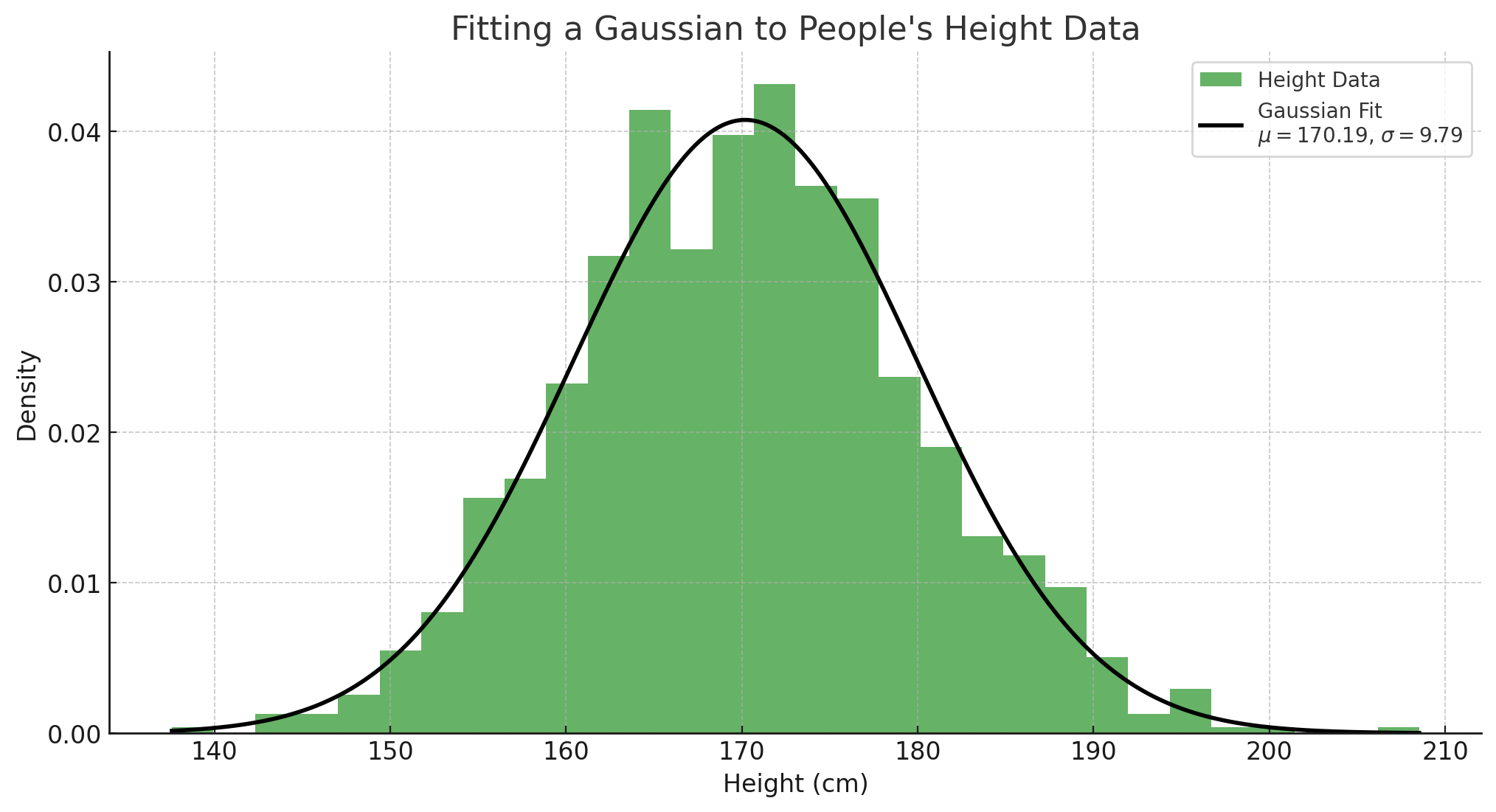
In this section, we visualize the process of fitting a Gaussian distribution to a dataset of heights. The goal is to estimate the mean ($\mu$) and standard deviation ($\sigma$) of the heights in the population.

The mean represents the average height, while the standard deviation indicates how much the heights vary from the mean. By fitting a Gaussian distribution, we can see how well our model captures the underlying data distribution. The curve illustrates the probability density function of the fitted normal distribution, showing the likelihood of different height values occurring in the population. This foundational concept is crucial for understanding more complex generative models that build upon the principles of normal distributions.

The loss landscape here will be a two dimensional one, with the two dimensions being the mean and the variance. We could do gradient descent on this landscape to find the optimal parameters, but we can actually find with a bit of maths that we end up with the closed form solution for the mean and variance. It’s worth trying to do this, hint take the gradient and set it to 0, then solve for \(\mu\) and \(\sigma\).

The Manifold Hypothesis

In high-dimensional spaces (like an image), data rarely lies in a simple Gaussian distribution, instead it’s in a much more complex distribution. The manifold hypothesis is a key idea in generative modeling, suggesting that high-dimensional data (like images or audio) lies on a lower-dimensional manifold (surface) embedded within the high-dimensional space. An intuitive way to think about is this is that there many combinations of pixels that form an image, but only some of those combinations look like images.

For example: A 64x64 image of a face lives in a 4,096-dimensional space, but the set of all possible human faces occupies a much smaller subspace. Generative models aim to learn this underlying manifold and generate new samples that also lie on it. This hypothesis is crucial for models like GANs and VAEs, which seek to capture the data’s latent structure - the underlying characteristics such as shape, colour, etc, and not just the pixel values.

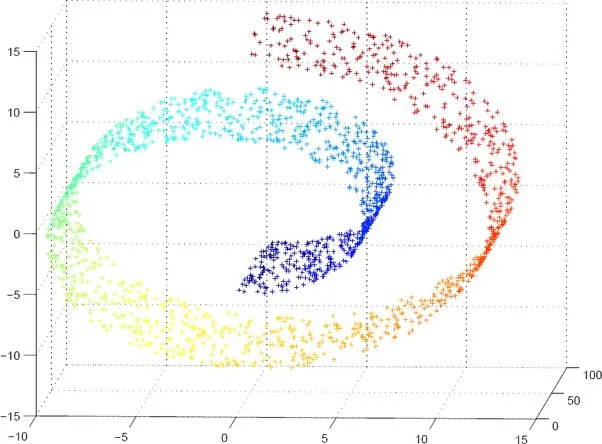
This image illustrates the manifold hypothesis, which shows that high-dimensional data lies on a lower-dimensional manifold within the high-dimensional space. i.e. a 2d plane in a 3d space.

Generative Adversarial Networks (GANs)

GANs, introduced by Goodfellow et al. in 2014, are a class of generative models that learn to generate data by playing a minimax game between two neural networks:

• Generator (G): Generates fake samples from random noise.
• Discriminator (D): Distinguishes between real and fake samples.

Objective Function (Minimax Game): The goal is to learn a generator that fools the discriminator and a discriminator that can tell the difference between a real and fake images, this is basically an arms race. The GAN objective can be expressed as: \(\min_G \max_D \mathbb{E}_{x \sim p_{data}} [\log D(x)] + \mathbb{E}_{z \sim p_z} [\log (1 - D(G(z)))]\)

We basically try and train both the generator and discriminator to get better at their respective tasks. The generator is trying to generate samples that are indistinguishable from the real data, while the discriminator is trying to correctly classify real and fake samples. You might have noticed that the descriminator is using the Binary Cross Entropy loss, while the generator if folliwng the example above.

Lipschitz Continuity and WGANs:

A significant challenge with GANs is training stability. As we spoke about last time, this is caused by loss landscape not being smooth enough, leading to exploding gradients. To get around this, we can enforce the Lipschitz (basically tells you the maximum gradient) constraint on the discriminator. This is done by clipping the weights of the discriminator, or using a gradient penalty.

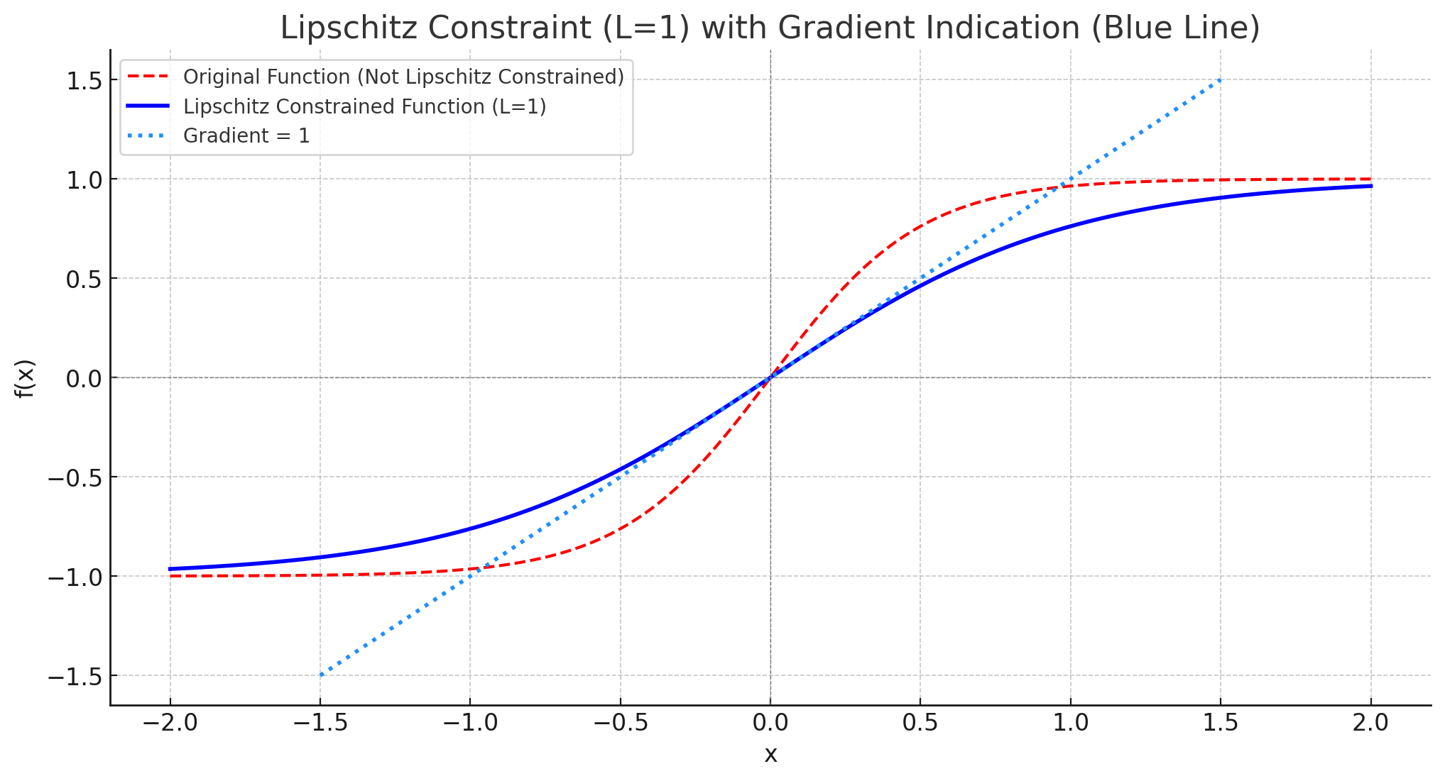
Lipschitz continuit is important as the gradients are bounded, if a function is Lipschitz continuous with a constant ( L ), it means that the absolute value of the gradient is at most ( L ). In our case, if we enforce a Lipschitz constraint of 1, it implies that the gradients of the discriminator in the GAN setup cannot exceed 1. This helps in stabilizing the training process, preventing issues like exploding gradients, and ensures that the updates to the model parameters remain controlled and manageable, i.e we don’t fall of a cliff.

Improved Techniques for GANs:

• WGAN: A method that enforces the Lipschitz constraint by clipping the weights of the discriminator.
• WGAN-GP: A smooth way to enforce the Lipschitz constraint, i.e. we don’t do hard clipping.
• Spectral Normalization: Ensures Lipschitz continuity by normalizing the spectral norm of each layer.
• Orthogonal Weights: Use orthogonal weights, this is isn’t neceesarily related to Lipshitz, but it helps keep the samples diverse by stopiing the representations collapsing to a lower dimensional feature space (i.e. we have many more features to play with).

Variational Autoencoders (VAEs)

Variational Autoencoders (VAEs) are another type of generative models that combine probabilistic modeling with neural networks. Unlike GANs, which generate data adversarially, VAEs take a probabilistic approach to model the latent space, i.e. they try and fit a distribution to the data, but also try and learn the latent factors. The core idea is to encode input data into a probabilistic distribution over a latent space and then decode it back to generate samples. This is a great example of how we want to map from the simple distribution containing the latent factors to the complex distribution containing the data.

Key Concepts in VAEs

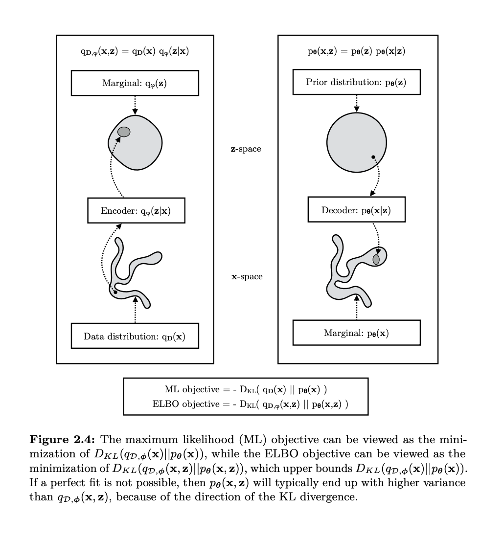
The Evidence Lower Bound (ELBO)

The VAE maximizes a lower bound on the data likelihood known as the Evidence Lower Bound (ELBO). We can derive the ELBO like so:

1. Start with the definition of the marginal likelihood, i.e. margincalize out \(z\): \(p(x) = \int p(x|z) p(z) dz\)

2. Introduce an approximate posterior \(q(z \mid x)\): \(p(x) = \int q(z|x) \frac{p(x|z) p(z)}{q(z|x)} dz\)

3. Apply Jensen’s inequality (this is where the lower bound comes in): \(\log p(x) \geq \mathbb{E}_{q(z|x)}\left[\log \frac{p(x|z) p(z)}{q(z|x)}\right]\)

4. This can be rewritten as: \(\log p(x) \geq \mathbb{E}_{q(z|x)}[\log p(x|z)] - D_{KL}(q(z|x) || p(z))\)

5. Thus, we arrive at the final form of the ELBO: \(\log p(x) \geq \mathbb{E}_{q(z|x)}[\log p(x|z)] - D_{KL}(q(z|x) || p(z))\)

Here, \(q(z\mid x)\) is the approximate posterior, and \(D_{KL}\) is the Kullback-Leibler divergence, which penalizes deviations of \(q(z\mid x)\) from the prior \(p(z)\). The reconstruction term encourages accurate reconstructions of the input, while the KL divergence term ensures a structured latent space. Mechanistically, we first encode \(\x\) through \(q(z\mid x)\), which is a neural network that predicts a meand and variance, we sample from this Gaussian distribution and then reconstruct the sample. We then take the mean squared error between the input \(x\) and the the output form the decoder, which is just summing up the difference between the pixels, taking the square and then dividing by the number of pixels.

Variance of the Estimators and Gradient Stability

In the context of VAEs, high variance in the gradient estimate to the encoder arise when sampling from the approximate posterior \(q(z|x)\), as it’s a stochastic process (think about randomly changing your directioin while walking down the hill). Since backpropagation cannot flow through random sampling, techniques like REINFORCE or the reparameterization trick are necessary to ensure stable training.

REINFORCE and Variance in Gradient Estimators

REINFORCE is a fundamental algorithm in reinforcement learning (Williams, 1992) but is also applicable in probabilistic models like VAEs. It provides an unbiased gradient estimator for expectations over stochastic processes, but this estimator often suffers from high variance, making training challenging and unstable.

For a probability distribution parameterized by \(\theta\), the goal is to compute the gradient of an expectation:

(For a VAE we’re trying to compute the gradient of the ELBO, so we’re trying to compute the gradient of the expectation of the log likelihood of the data under the model. Using the log-derivative trick, REINFORCE estimates the gradient as:

This is an unbiased estimator (i.e. on average it gets to the true value), but the variance of the estimator can still be very high.

The Reparameterization Trick

This is the most common solution to high variance in VAEs, transforming the stochastic sampling process into a deterministic one by introducing auxiliary noise:

By reparameterizing, gradients can propagate through \(\mu(x)\) and \(\sigma(x)\) directly, i.e. we take the gradient of the mean and variance directly and not the same, this reduces the variance and allows us to train the model.

Variance Reduction with Control Variates

Borrowing from reinforcement learning, control variates can further reduce variance. A baseline function can be subtracted from the reward signal without introducing bias, stabilizing training. For example, a learned value function \(b(x)\) can serve as a baseline:

KL Annealing

Gradually increasing the weight of the KL divergence term (annealing) during early training prevents the model from collapsing the latent space too soon (posterior collapse), leading to more stable and meaningful representations.

Intepretability of VAEs

One of the main reason people like VAEs is that we can use the latent space to interpret features of the data. For example, if we have a VAE that models human faces, we can use the latent space to understand how different features of the face are related to each other. We can also change the latent factors and directly cause certain features to change in the image. This can be seen in the image below:

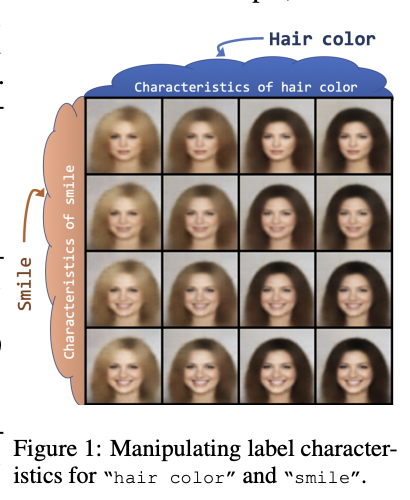
This is really useful when compared to GANs, as we can now theoretically control conceptual factors of the image by altering certain parts of the latent space.

Invertible Neural Networks (INNs)

Invertible Neural Networks (INNs) focus on learning bijective (one to one) transformations between the data space and the latent space. Unlike VAEs and GANs, INNs ensure exact likelihoods. They are similar to the VAE in that they map compelx data to a latent space, but they are different in that they are invertible, i.e. there is not fixed decoder/encoder, it is just one network that maps forwards and backwards. They start by modelling a change of variables:

which when taking the log for high dimensional data, we get:

where $z$ is the latent space and $x$ is the data space, and the final term is the log determinant of the Jacobian matrix of the transformation.

• Rank and Lipschitz Constraints: As we are dealing with Jacobians (gradient of all outputs wrt to all inputs), we need to ensure that the transformation is bijective, i.e. one-to-one and invertible. Controlling the Lipschitz constant helps maintain stability and ensures smooth transformations. A great way to do this is through the use of ResNets, which due to their skip connections are always full rank and invertible. Check out the paper Invertible Residual Networks for more details.

Summary

Each of these generative models—GANs, VAEs, and INNs—offers unique advantages and challenges. The choice of model depends on the task at hand:

• GANs are best for generating high quality images (pre diffusion models).
• VAEs are best for finding the latent features.
• INNs offer exact computation of the likelihood.

Most of these methods are now obsolete, and have been replaced by more powerful methods such as diffusion models, which we will cover next time.